Table of Contents
The QSM plug-in provides a set of additional descriptors. Most of them are taken from “Hackenberg, Jan, and Jean-Daniel Bontemps.”Improving quantitative structure models with filters based on allometric scaling theory.” Applied Geomatics 15.4 (2023)“.
The shoot based descriptors can be taken from the QSM inspector or can be used in RGG with its descriptor key, as following:
import static  de.grogra.qsm.utils.Descriptors.*;

...

public void test(){
    println((*F[GROWTH_LENGTH]*)); //print all growth length in the XL console
    println(sum((*F[GROWTH_LENGTH]*))); //print sum of all growth length in the XL console
    [
        f:F,(f[TIP]) ==>f Sphere(0.01); // add a sphere on top of each tip of the tree.
    ]
}
Following common assumption, we consider a branch to be a chain of apically linked shoots. Every lateral shoot describes a new branch, which is a child branch of the branch of the parent shoot of the new shoot. To display the different relationships in a GroIMP graph, successor and branch edges are used. A apical shoot is linked to its parent with a successor edge and a lateral shoot with a branch edge. Following the concept of QSM and tree taxonomy we assume each shoot can only have one apical child and therefore each shoot can only have one successor (the child connected with a successor edge).
For each shoot the branch order describes the taxonomical distance from the branch of this shoot to the root of the tree. Therefore the trunk has a branch oder of 0, the branches emerging from the trunk a branch oder of 1.
descriptor key:
(*F*)[BO]
Formal definition:
The branch order of a shoot s1 is described as following:
BO(s1) = BO(axisParent(s1)) + 1
axisParent(s1) returns the shoot from which the branch of s1 was laterally emerged. (This is a GroIMP core function: javadoc )
The reverse branch order of a shoot describes the highest number of continuously connected branches emerging from this shoot.
descriptor key:
(*F*)[RBO]
Formal definition:
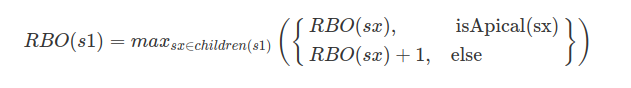
children(s1) describes all shoots directly connected to s1 with s1 as source.
isApical(sx) is true if the incomming connectio is a successor edge. (the shoot is the apical child / on the same branch)
The trend of a shoot describes its position on the branch based on the number of shoots preceding it on the same branch.
descriptor key:
(*F*)[TREND]
Formal definition:
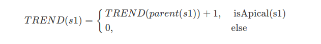
isApical(sx) is true if the incomming connectio is a successor edge. (the shoot is the apical child / on the same branch)
parent(s1) represents the node that is connected to s1 with s1 as target.
Analog to the trend the reverse trend describes the position of a shoot on its branch based on the number of shoots succeeding it on the same branch.
descriptor key:
(*F*)[RTREND]
Formal definition:
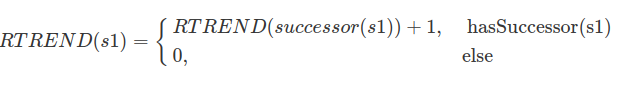
parent(s1) represents the node that is connected to s1 with s1 as target.
hasSuccessor(s1) is true if one of the children of s1 is linked by successor edge.
The root distance of a shoot is the number of shoots preceding it in.
descriptor key:
(*F*)[ROOT_DISTANCE]
Formal definition:
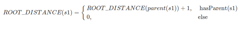
parent(s1) represents the node that is connected to s1 with s1 as target.
hasParent(s1) is true if s1 has an incoming edge.
The number of direct children (both apical and lateral) of a given shoot.
descriptor key:
(*F*)[CHILD_COUNT]
Formal definition:
CHILD_COUNT(s1) = |children(s1)|
children(s1) describes all shoots directly connected to s1 with s1 as source.
A Tip describes a shoot without any children, in terms of a mathematical tree graph it is considered a leaf.
descriptor key:
(*F*)[TIP]
Formal definition:
if CHILD_COUNT(s1) is 0.
A Shoot is considered an apical tip if it has no apical child.
descriptor key:
(*F*)[ATIP]
Formal definition:
if !hasSuccessor(s1).
hasSuccessor(s1) is true if one of the children of s1 is linked by successor edge.
The number of shoots on the longest ongoing path from the given shoot to a tip.
descriptor key:
(*F*)[MAX_TIP_DISTANCE]
Formal definition:
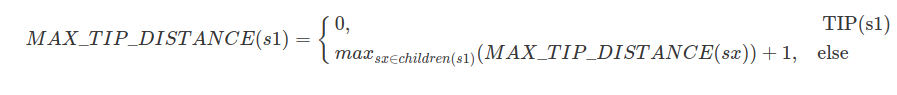
children(s1) describes all shoots directly connected to s1 with s1 as source.
The number of shoots on the shortest ongoing path from the given shoot to a tip.
descriptor key:
(*F*)[MIN_TIP_DISTANCE]
Formal definition:
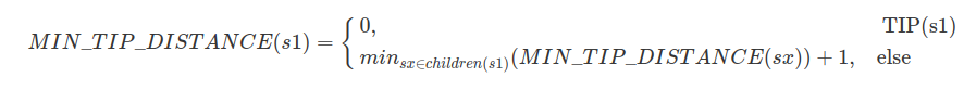
children(s1) describes all shoots directly connected to s1 with s1 as source.
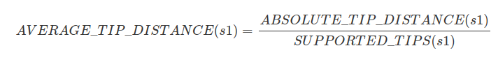
The sum of the number of shoots all paths form the given shoot to every tips. Since every path starts at the same position, shoots are counted for each tip they are supporting.
descriptor key:
(*F*)[ABSOLUTE_TIP_DISTANCE]
Formal definition:
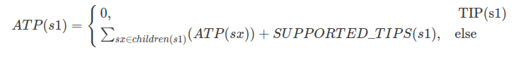
children(s1) describes all shoots directly connected to s1 with s1 as source.
The growth length (introduces by Hackenberg et al.) describes sum of the length of all shoots following the given shoot and the shoot it self.
descriptor key:
(*F*)[GROWTH_LENGTH]
Formal definition:
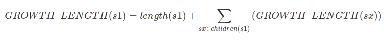
children(s1) describes all shoots directly connected to s1 with s1 as source.
The amount of tips following the given shoot, in Hackenberg et al. this as the Reverse Branch Order Pipe Area.
descriptor key:
(*F*)[SUPPORTED_TIPS] or
(*F*)[RBOPA]
Formal definition:
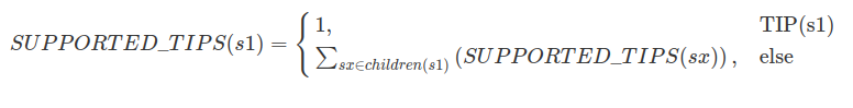
children(s1) describes all shoots directly connected to s1 with s1 as source.
The proxy volume (Hackenberg et al.) describes the assumed volume of a shoot using the Reverse Branch Order Pipe Area as the cut trough area of the shoot.
descriptor key:
(*F*)[PROXY_VOLUME]
Formal definition:
PROXY_VOLUME(s1) = RBOPA(s1) * length(s1)
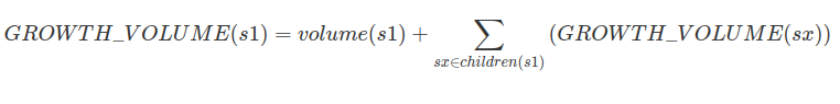
The Vessel volume (Hackenberg et al.) is calculated analog to the growth volume but based on the proxy volume.
descriptor key:
(*F*)[VESSEL_VOLUME]
Formal definition:
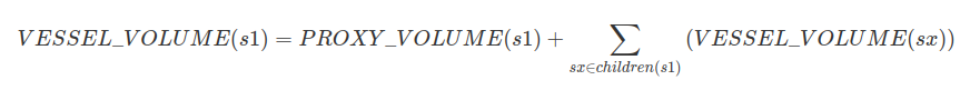
children(s1) describes all shoots directly connected to s1 with s1 as source.
Based on the number of supported tips and the average cross section area of a tip a pipe model can be applied to estimate the sap wood of a shoot.
Following the idea of a pipe model the cross section area of sap wood of a branch is the sum of the cross section area of the supported tips, to simplify the approach at this place, the average cross section area of the tips is used.
descriptor key:
(*F*)[SAPWOOD_AREA]
Formal definition:
SAPWOOD_AREA(s1) = SUPPORTED_TIPS(s1) * average_tip_area
average_tip_area a tree wide descriptor
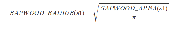
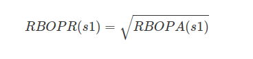
The radius based on the estimated sap wood area
descriptor key:
(*F*)[SAPWOOD_RADIUS]
Formal definition: